
Contents
- The difference at a glance
- Start with a forecast, not a yes-or-no pick
- The same three forecasts, scored both ways
- Why two Brier scores can differ by a factor of two
- Log base, zero probabilities and clipping
- What “strictly proper” does, and does not, promise
- A fair comparison checklist
- What neither score tells you on its own
- Sources
Brier score and log loss both measure the quality of probability forecasts, with lower loss meaning better performance. The practical difference is how they treat a confident mistake: binary Brier loss is bounded, while log loss grows without limit as the probability assigned to the outcome that happens approaches zero.
Use Brier score when you want an easy-to-read squared-error measure. Use log loss when you want the evaluation to be especially sensitive to near-impossible predictions that turn out to happen. For a forecast comparison, reporting both can be useful, but choose your primary measure before looking at the results. Their raw numbers are not interchangeable.
Before comparing two published scores, check four details: Brier scaling, logarithm base, averaging and any probability clipping. Otherwise, the same forecasts can appear to have different performance simply because the calculations use different conventions.
The difference at a glance
| Question | Brier score | Log loss |
|---|---|---|
| What does it calculate? | Squared differences between probabilities and outcomes | Negative logarithm of the probability assigned to the observed outcome |
| What does a perfect forecast score? | 0 | 0 before clipping |
| What is the range? | 0–1 for the binary convention used here; 0–2 for the full class-sum convention | 0 to positive infinity for discrete outcomes |
| What happens to an overconfident miss? | The loss approaches its finite maximum | The loss grows without a finite upper bound |
| What must you label? | Binary or full class-sum scaling | Logarithm base and endpoint treatment |
These are loss conventions: smaller is better. A source that reports the logarithmic score with the opposite sign reverses that direction. The scoringrules theory guide explains both the loss convention and why the choice of scoring rule can change a ranking.
Start with a forecast, not a yes-or-no pick
Suppose you forecast a clearly defined event, such as whether a team will win a match under specified rules. Let p be your probability of “yes,” and let y equal 1 if “yes” happens or 0 otherwise. The probability of “no” is 1 − p.
A prediction of 51% and one of 99% both select “yes,” but express very different confidence. If “yes” happens, their binary Brier losses are 0.2401 and 0.0001. A right-or-wrong tally would miss that distinction.
For one binary forecast:
- Binary Brier loss = (p − y)².
- Natural-log loss = −ln(p) when y = 1, or −ln(1 − p) when y = 0.
For probabilities strictly between 0 and 1, the second formula is also written −[y ln(p) + (1 − y) ln(1 − p)]. The branch form makes endpoint handling clearer. Across N equally weighted forecasts, add the individual losses and divide by N. These definitions follow the Brier score documentation and log-loss documentation.
The same three forecasts, scored both ways
This hypothetical dataset contains three equally weighted forecasts recorded before their outcomes. It is a teaching example, not a platform track record. Each event has a fixed yes/no definition and a resolved outcome. The main calculation uses no clipping.
| Event | Forecast p(yes) | Outcome y | Binary Brier loss | Natural-log loss |
|---|---|---|---|---|
| A | 0.80 | 1 | 0.040000 | 0.223144 |
| B | 0.30 | 0 | 0.090000 | 0.356675 |
| C | 0.01 | 1 | 0.980100 | 4.605170 |
| Mean | 0.370033 | 1.728330 |
Event B uses −ln(0.70), because “no” was the observed outcome. Event C assigned only 1% to an outcome that happened, so it receives a large loss under both rules.
The binary Brier mean is (0.04 + 0.09 + 0.9801) ÷ 3 = 0.370033, rounded to six decimal places. The natural-log mean is [−ln(0.80) − ln(0.70) − ln(0.01)] ÷ 3 = 1.728330. All means are calculated from unrounded values.
The lower numerical value of the Brier mean does not make Brier the “better” result. You can compare one forecaster's Brier score with another forecaster's Brier score on the same events and convention. Comparing 0.370033 directly with 1.728330 mixes two different scales.
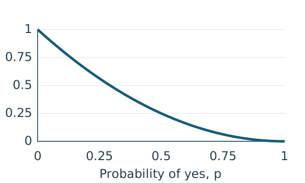
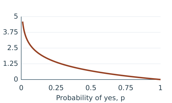
What the penalty curves show
For a fixed outcome of “yes,” increasing p reduces either loss. Near zero, however, the curves behave differently. Brier approaches 1; natural-log loss keeps rising.
Binary Brier loss
Outcome: yes. Formula: (1 − p)². Vertical scale: 0–1.
Natural-log loss
Outcome: yes. Formula: −ln(p). Vertical scale: 0–5.
| Probability of “yes,” when yes happens | Binary Brier loss | Natural-log loss |
|---|---|---|
| 0.50 | 0.250000 | 0.693147 |
| 0.10 | 0.810000 | 2.302585 |
| 0.01 | 0.980100 | 4.605170 |
| 0.00 | 1.000000 | Positive infinity, without clipping |
Brier remains responsive to confident errors; it simply limits each event's contribution. Log loss has no such ceiling. That distinction matters when a small number of very confident misses might drive an overall result.
Why two Brier scores can differ by a factor of two
The binary formula above scores only the probability of “yes.” Another convention sums squared errors across every class. For a two-class event, it includes both “yes” and “no”:
Full class-sum Brier loss = (p − y)² + [(1 − p) − (1 − y)]² = 2(p − y)².
The three-event mean therefore becomes 0.740067 under the full class-sum convention, rather than 0.370033 under the binary convention. Nothing about the forecasts changed. Doubling every score preserves the ranking when every forecast is scored on that same basis.
For mutually exclusive and collectively exhaustive classes, the full class-sum Brier range is 0–2. Dividing that score by two gives a 0–1 range. The scikit-learn Brier documentation describes this scaling distinction. Check the convention explicitly rather than inferring it from the label “Brier score.”
A three-outcome example
Suppose a hypothetical event has exactly three possible outcomes, A, B and C, with probabilities 0.70, 0.20 and 0.10. They sum to 1. If A happens, the outcome vector is (1, 0, 0).
| Outcome | Forecast probability | Observed outcome indicator | Squared error |
|---|---|---|---|
| A | 0.70 | 1 | 0.09 |
| B | 0.20 | 0 | 0.04 |
| C | 0.10 | 0 | 0.01 |
The full class-sum Brier loss is 0.09 + 0.04 + 0.01 = 0.14. If explicitly scaled by one-half, it is 0.07. Do not average the three class errors and call that the same convention.
Categorical log loss uses the probability of the class that happened: −ln(0.70) = 0.356675. It does not add a separate −ln(1 − p) term for every losing class. See the categorical scoring-rule definitions.
This example covers a single event with one winning class. A collection of labels that can all occur together requires a different event setup, not an automatic reuse of this categorical formula.
Log base, zero probabilities and clipping
Changing the base changes the number, not the ranking
Here, ln means the natural logarithm, with base e. With base-2 logarithms instead, divide the natural-log loss by ln(2). The three-event mean becomes 2.493452, rather than 1.728330. This is a positive rescaling, so rankings are unchanged when every forecast uses the same base.
The scikit-learn log-loss documentation specifies natural logarithms. If you compare output from different tools or publications, also check whether each reports a mean or a sum and whether sample weights are applied.
A certain prediction has two very different endpoints
Without clipping, assigning probability 1 to the outcome that happens produces zero log loss. Assigning probability 0 to that outcome produces positive infinity. For binary Brier loss, those cases score 0 and 1 respectively.
In the expanded log-loss formula, use the usual limiting convention for terms such as 0 × ln(0), or evaluate the probability of the observed class directly. Do not treat an undefined numerical operation as evidence that the mathematical endpoint is missing.
Software often clips probabilities away from 0 and 1 to avoid infinite numerical results. As an explicit teaching choice, let ε = 0.000001 and replace a binary probability p with min(1 − ε, max(ε, p)). If p was 0 and “yes” happens, the clipped log loss is −ln(0.000001) = 13.815511 instead of infinity.
That ε is not a claim about a library default. The scikit-learn documentation describes clipping based on the probability array's numeric data type; implementation details should be checked against the version you actually run. Clipping also changes the score being evaluated: forecasts beyond the same clipping boundary become indistinguishable. Keep the original probabilities, disclose the threshold and report how often clipping occurred.
What “strictly proper” does, and does not, promise
Under their mathematical definitions, Brier and log loss are strictly proper scoring rules. In expectation, the unique best forecast is the true probability distribution. This property discourages changing a genuinely held probability merely to improve the expected score. It does not promise the best score on every small sample. Scoring-rule theory makes this expectation-based distinction explicit.
For a binary event with true probability q, expected Brier loss can be written:
Expected loss = q(1 − p)² + (1 − q)p² = q(1 − q) + (p − q)².
If q = 0.70, forecasting p = 0.70 gives expected loss 0.21. Forecasting p = 0.90 gives 0.25. Yet if the next outcome happens to be “yes,” the 90% forecast earns a lower loss on that one event. The expected result and the realized result answer different questions.
Clipping needs its own qualification. Strict propriety of the original rule does not mean an implementation that maps several submitted probabilities to the same clipped value can uniquely reward all those original probabilities.
A fair comparison checklist
Before choosing a forecaster or claiming an improvement, make the comparison reproducible:
- Match the question and outcome rules. Define the event, deadline, class labels and resolution source. For a match, “wins in regulation time” and “qualifies after extra time” are different events. Decide in advance how void, disputed or unresolved events will be handled.
- Match forecast timing. Compare forecasts made with comparable information and time remaining. Do not compare an early forecast from one source with a near-resolution update from another without explaining that difference.
- Match the evaluation set. Use the same resolved events, report the count and identify missing forecasts. Choosing different easy or difficult events can make an aggregate comparison misleading.
- Declare the arithmetic. State the Brier scaling, log base, mean or sum, weights, clipping and class order. A weighted mean is Σ(wᵢ × lossᵢ) ÷ Σwᵢ for nonnegative weights with a positive total. Explain what those weights represent.
- Keep evaluation separate from fitting. Assess performance on outcomes not used to fit or tune the forecasting method. If forecasts are repeatedly updated, specify whether you score one fixed snapshot per event or several snapshots and how you weight them.
- Use a stated reference forecast. Compare with a baseline chosen in advance and report its construction. An always-50% forecast has binary Brier loss 0.25 and natural-log loss 0.693147 on every binary event, but it is not necessarily an informative baseline for an imbalanced event set.
This is an evaluation protocol, not a universal score threshold. A small observed advantage is a result for that sample, not automatic evidence of a durable advantage.
What neither score tells you on its own
Calibration: If forecasts near 70% are well calibrated, roughly 70% of those events should happen over a suitable collection of cases. A lower Brier score alone does not establish better calibration: the score also reflects how well forecasts distinguish outcomes and the uncertainty in the data. Use a calibration curve with enough observations and visible bin counts alongside the aggregate score. The scikit-learn calibration guide explains this limitation.
Profitability: Neither formula contains a trade's entry price, stake, fees, liquidity or exit decision. A lower forecast loss therefore does not, by itself, establish a profitable trading strategy. Evaluating a forecast and evaluating a trade require different records.
Universal quality: A score has meaning relative to its rule, event set and reference forecast. Neither the three-event example nor a single favorable number proves that a platform is accurate across markets.
The useful next step is simple: keep the forecasts and outcomes together, declare the scoring convention, and compare like with like. Brier gives you a bounded squared-error view; log loss makes near-zero probabilities for observed outcomes particularly consequential. Read the scores together with timing, sample coverage and calibration rather than treating either as a complete verdict.
Continue learning
Choose another explanation for the question you want to check next.
Sources
- scikit-learn: Brier score loss, binary and full class-sum definitions and scaling.
- scikit-learn: Log loss, natural-log formula, aggregation and numerical treatment.
- scoringrules: The theory of proper scoring rules, propriety in expectation and categorical scoring.
- scikit-learn: Probability calibration, calibration curves and limits of aggregate loss as a calibration measure.
HypaForecast publishes educational guides and operates a prediction market. This page is an educational explanation.
Share this guide